第 2 章单样本位置参数

2.1 引入的例子：楼盘均价

##数据
x1 <- c(36, 32, 31, 25, 28, 36, 40, 32, 41, 26, 35, 35, 32, 87, 33, 35)
##单样本t检验
t.test(x1,mu=37)

## 
##  One Sample t-test
## 
## data:  x1
## t = -0.14123, df = 15, p-value = 0.8896
## alternative hypothesis: true mean is not equal to 37
## 95 percent confidence interval:
##  28.95415 44.04585
## sample estimates:
## mean of x 
##      36.5

##直方图
hist(x1)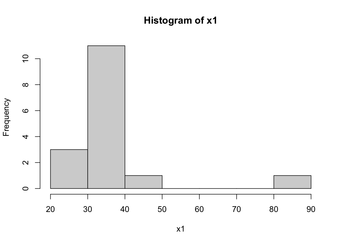

##向量计算
x1-37

##  [1]  -1  -5  -6 -12  -9  -1   3  -5   4 -11  -2  -2  -5  50  -4  -2

(x1<37)

##  [1]  TRUE  TRUE  TRUE  TRUE  TRUE  TRUE FALSE  TRUE FALSE  TRUE  TRUE  TRUE
## [13]  TRUE FALSE  TRUE  TRUE

##sign test
library(BSDA)

## Loading required package: lattice

## 
## Attaching package: 'BSDA'

## The following object is masked from 'package:datasets':
## 
##     Orange

SIGN.test(x1,md=37,alternative="two.sided",conf.level=0.95)

## 
##  One-sample Sign-Test
## 
## data:  x1
## s = 3, p-value = 0.02127
## alternative hypothesis: true median is not equal to 37
## 95 percent confidence interval:
##  31.51725 36.00000
## sample estimates:
## median of x 
##          34 
## 
## Achieved and Interpolated Confidence Intervals: 
## 
##                   Conf.Level  L.E.pt U.E.pt
## Lower Achieved CI     0.9232 32.0000     36
## Interpolated CI       0.9500 31.5173     36
## Upper Achieved CI     0.9787 31.0000     36

检验统计量\(S=\min\{S^+,S^-\}\),\(S^+=\#\{X>median\}\),\(S^-=\#\{X<median\}\);
\(n=s^++s^-\);
p值=\(2P(S\leq s)\)，\(S \sim B(n,0.5)\)

2*(1-pbinom(12,16,0.5)) #2P(S>=n-s)=2P(S>=13)=2[1-P(S<=12)]

## [1] 0.02127075

2*pbinom(3,16,0.5) #2P(S<=s)=2P(S<=3)

## [1] 0.02127075

##wilcoxon signed rank test
wilcox.test(x1,mu=37,alternative="two.sided")

## Warning in wilcox.test.default(x1, mu = 37, alternative = "two.sided"): cannot
## compute exact p-value with ties

## 
##  Wilcoxon signed rank test with continuity correction
## 
## data:  x1
## V = 29.5, p-value = 0.04904
## alternative hypothesis: true location is not equal to 37

2.2 2.1 符号检验 Sign Test

2.2.1 2.1.1. 广义符号检验

2.2.1.1 SIGN.test只能处理中位数的问题

expens <- read.table(file="data/ExpensCities.TXT")
SIGN.test(expens$V1,md=64,alternative="two.sided",conf.level=0.95)

## 
##  One-sample Sign-Test
## 
## data:  expens$V1
## s = 43, p-value = 0.09592
## alternative hypothesis: true median is not equal to 64
## 95 percent confidence interval:
##  63.28094 77.04644
## sample estimates:
## median of x 
##        67.7 
## 
## Achieved and Interpolated Confidence Intervals: 
## 
##                   Conf.Level  L.E.pt  U.E.pt
## Lower Achieved CI     0.9432 63.5000 76.8000
## Interpolated CI       0.9500 63.2809 77.0464
## Upper Achieved CI     0.9681 62.7000 77.7000

2.2.1.2 自定义函数：广义符号检验

sign.test=function(x,p,q0){
  s1=sum(x<q0);s2=sum(x>q0);n=s1+s2
  p1=pbinom(s1,n,p);p2=1-pbinom(s1-1,n,p)
  if (p1>p2){
    m1="One tail test: H1: Q<q0"
  }
  else{
    m1="One tail test: H1: Q>q0"
  }
  p.value=min(p1,p2);m2="Two tails test";p.value2=2*p.value
  if (q0==median(x)){
    p.value=0.5;p.value2=1
  }
  list(Sign.test1=m1, p.values.of.one.tail.test=p.value,
  p.value.of.two.tail.test=p.value2)
}

sign.test(expens$V1,0.5,64)

## $Sign.test1
## [1] "One tail test: H1: Q>q0"
## 
## $p.values.of.one.tail.test
## [1] 0.04796182
## 
## $p.value.of.two.tail.test
## [1] 0.09592363

sign.test(expens$V1,0.25,64)

## $Sign.test1
## [1] "One tail test: H1: Q<q0"
## 
## $p.values.of.one.tail.test
## [1] 0.005151879
## 
## $p.value.of.two.tail.test
## [1] 0.01030376

\(H_0:Q_{0.25} \geq 64 \leftrightarrow H_1:Q_{0.25} < 64\);
检验统计量\(S^-=\#\{X<q_0\}\),\(q_0=64\),\(n=s^++s^-\);
如果\(Q_{0.25} = q_0\)，应有\(S^- \sim B(n,0.25)\);
如果\(s^-\)的值较大，说明较多的值比\(q_0\)小，因此\(Q_{0.25} < q_0\);
此时，p值\(=P(S\geq s^-)=1-P(S\leq s^--1)\)，\(S \sim B(n,0.25)\)

2.2.2 2.1.2 分位点的置信区间

2.2.2.1 中位数的置信区间

tax <- read.table(file="data/tax.TXT")
(tax <- sort(tax$V1))

##  [1] 1.00 1.35 1.99 2.05 2.05 2.10 2.30 2.61 2.86 2.95 2.98 3.23 3.73 4.03 4.82
## [16] 5.24 6.10 6.64 6.81 6.86 7.11 9.00

SIGN.test(tax,alternative="two.sided",conf.level=0.95)$Confidence.Intervals

##                   Conf.Level L.E.pt U.E.pt
## Lower Achieved CI     0.9475 2.3000 5.2400
## Interpolated CI       0.9500 2.2861 5.2999
## Upper Achieved CI     0.9831 2.1000 6.1000

2.2.2.2 自定义函数（一）：中位数的置信区间

mci=function(x,alpha=0.05){
  n=length(x)
  b=0
  i=0
  while(b<=alpha/2&i<=floor(n/2)){
    b=pbinom(i,n,.5);
    k1=i;k2=n-i+1;
    a=2*pbinom(k1-1,n,.5);
    i=i+1
  }
  z=c(k1,k2,a,1-a);
  z2="Entire range!"
  if(k1>=1){
    out=list(Confidence.level=1-a,CI=c(x[k1],x[k2]))
  }
  else{
    out=list(Confidence.level=1-2*pbinom(0,n,.5),CI=z2)
  }
  out
}
mci(tax,alpha=0.05)

## $Confidence.level
## [1] 0.9830995
## 
## $CI
## [1] 2.1 6.1

2.2.2.3 自定义函数（二）：中位数的置信区间

mci2=function(x,alpha=0){
  n=length(x);q=.5
  m=floor(n*q);s1=pbinom(0:m,n,q);s2=pbinom(m:(n-1),n,q,low=F);
  ss=c(s1,s2);nn=length(ss);a=NULL;
  for(i in 0:m){
    b1=ss[i+1];b2=ss[nn-i];b=b1+b2;d=1-b;
  if((b)>1)break
    a=rbind(a,c(b,d,x[i+1],x[n-i]))}
  if(a[1,1]>alpha){
    out="alpha is too small, CI=All range"   
  } 
  else{
    for(i in 1:nrow(a)){
      if(a[i,1]>alpha){out=a[i-1,];break}
    } 
  }
  out
}
mci2(tax,alpha=0.05)

## [1] 0.01690054 0.98309946 2.10000000 6.10000000

2.2.2.4 分位数的置信区间

qci=function(x,alpha=0.05,q=.25){
  x<-sort(x);n=length(x);a=alpha/2;r=qbinom(a,n,q);
  s=qbinom(1-a,n,q);CL=pbinom(s,n,q)-pbinom(r-1,n,q)
  if (r==0) lo<-NA else lo<-x[r]
  if (s==n) up<-NA else up<-x[s+1]
  list(c("lower limit"=lo,"upper limit"=up,
        "1-alpha"=1-alpha,"true conf"=CL)) 
}
qci(tax,0.05,0.25)

## [[1]]
## lower limit upper limit     1-alpha   true conf 
##   1.3500000   2.9800000   0.9500000   0.9751605

qci(tax,0.06,0.25)

## [[1]]
## lower limit upper limit     1-alpha   true conf 
##    1.350000    2.950000    0.940000    0.955626

2.3 2.2 Wilcoxon符号秩检验(Wilcoxon Sign Rank)

2.3.1 2.2.1 检验

euroalc <- read.table(file="data/EuroAlc10.TXT")
y <- as.numeric(euroalc[1,])
y

##  [1]  4.12  5.81  7.63  9.74 10.39 11.92 12.32 12.89 13.54 14.45

wilcox.test(y-8)

## 
##  Wilcoxon signed rank exact test
## 
## data:  y - 8
## V = 46, p-value = 0.06445
## alternative hypothesis: true location is not equal to 0

wilcox.test(y-8,exact = F)

## 
##  Wilcoxon signed rank test with continuity correction
## 
## data:  y - 8
## V = 46, p-value = 0.06655
## alternative hypothesis: true location is not equal to 0

wilcox.test(y-8,alt="greater")

## 
##  Wilcoxon signed rank exact test
## 
## data:  y - 8
## V = 46, p-value = 0.03223
## alternative hypothesis: true location is greater than 0

wilcox.test(y-12.5,alt="less")

## 
##  Wilcoxon signed rank exact test
## 
## data:  y - 12.5
## V = 11, p-value = 0.05273
## alternative hypothesis: true location is less than 0

2.3.2 2.2.2 置信区间

2.3.2.1 Walsh平均

walsh=NULL;
for(i in 1:10){
  for(j in i:10){
    walsh=c(walsh,(y[i]+y[j])/2)
  }
} 
walsh=sort(walsh)
walsh

##  [1]  4.120  4.965  5.810  5.875  6.720  6.930  7.255  7.630  7.775  8.020
## [11]  8.100  8.220  8.505  8.685  8.830  8.865  9.010  9.065  9.285  9.350
## [21]  9.675  9.740  9.775  9.975 10.065 10.130 10.260 10.390 10.585 10.830
## [31] 11.030 11.040 11.155 11.315 11.355 11.640 11.640 11.920 11.965 12.095
## [41] 12.120 12.320 12.405 12.420 12.605 12.730 12.890 12.930 13.185 13.215
## [51] 13.385 13.540 13.670 13.995 14.450

2.3.2.2 利用Walsh平均构造置信区间

(k <- qsignrank(0.025,10))

## [1] 9

N <- length(walsh)
c(walsh[k+1],walsh[N-k])

## [1]  8.02 12.73

wilcox.test(y,conf.int = T)$conf.int

## [1]  7.775 12.890
## attr(,"conf.level")
## [1] 0.95

2.3.3 simulation study

Which of the two tests, the signed-rank Wilcoxon or the t-test, is the more powerful?

power_comparison <- function(mu){
  n = 30; df = 2; nsims = 10000; collwil = rep(0,nsims)
  collt = rep(0,nsims)
  for(i in 1:nsims){
    x = rt(n,df) + mu
    wil = wilcox.test(x)
    collwil[i] = wil$p.value
    ttest = t.test(x)
    collt[i] = ttest$p.value
  }
  powwil = rep(0,nsims); powwil[collwil <= .05] = 1
  powerwil = sum(powwil)/nsims
  powt = rep(0,nsims); powt[collt<= .05] = 1
  powert = sum(powt)/nsims
  list(powerwil,powert)
}
power_comparison(0)

## [[1]]
## [1] 0.049
## 
## [[2]]
## [1] 0.0371

power_comparison(0.5)

## [[1]]
## [1] 0.4584
## 
## [[2]]
## [1] 0.2868

power_comparison(1)

## [[1]]
## [1] 0.9195
## 
## [[2]]
## [1] 0.7023

2.4 2.3 正态记分检验*(normal score)

线性符号秩统计量 \(S_n^+=\sum_{i=1}^n a_n^+(R_i^+) I(X_i>0)\)；
- \(a_n^+(i)=i\)时，\(S_n^+\)为Wilcoxon符号秩统计量\(W^+\)；
- \(a_n^+(i)=1\)时，\(S_n^+\)为符号秩统计量\(S^+\)；
线性秩统计量 \(S_n=\sum_{i=1}^n c_n(i) a_n(R_i)\)；
- \(N=m+n\),\(a_N(i)=i\),\(c_N(i)=I(i>m)\),则\(S_n\)为两样本Wilcoxon秩和统计量;
- 正态记分\(S_n=\sum_{i=1}^n \Phi^{-1}\left( \frac{R_i}{n+1} \right)\);
线性秩统计量的一个特例 \(S_n=\sum_{i=1}^n a_n^+(R_i^+) sign(X_i)=\sum_{i=1}^n s_i\)；
- 记分函数\(a_n^+(i)=\Phi^{-1}\left( \frac{n+1+i}{2n+2} \right)=\Phi^{-1}\left[\frac{1}{2} \left( 1 + \frac{i}{n+1} \right) \right]\),非负
- 检验\(H_0:Me=M_0\),\(X_i-M_0\)的秩\(r_i\),符号正态记分\(s_i=a_n^+(r_i) sign(X_i-M_0)=\Phi^{-1}\left[\frac{1}{2} \left( 1 + \frac{r_i}{n+1} \right) \right]sign(X_i-M_0)\)

ns=function(x,m0){
  x1=x-m0;r=rank(abs(x1));n=length(x)
  s=qnorm(.5*(1+r/(n+1)))*sign(x1);
  tt=sum(s)/sqrt(sum(s^2));
  list(pvalue.2sided=2*min(pnorm(tt),pnorm(tt,low=F)),Tstat=tt,s=s)
}
ns(y,8)

## $pvalue.2sided
## [1] 0.05567649
## 
## $Tstat
## [1] 1.913559
## 
## $s
##  [1] -0.6045853 -0.3487557 -0.1141853  0.2298841  0.4727891  0.7478586
##  [7]  0.9084579  1.0968036  1.3351777  1.6906216

ns(y,12.5)

## $pvalue.2sided
## [1] 0.08114229
## 
## $Tstat
## [1] -1.744096
## 
## $s
##  [1] -1.6906216 -1.3351777 -1.0968036 -0.9084579 -0.7478586 -0.3487557
##  [7] -0.1141853  0.2298841  0.4727891  0.6045853

2.5 2.4 Cox-Stuart趋势检验*

判断增长或减少趋势
求差\(D_i=x_i-x_{i+c}\)的符号来衡量增减
像符号检验一样用到二项分布

TJair <- read.table(file="data/TJAir.TXT")
TJair <- as.vector(t(TJair))
plot.ts(TJair,xlab="Month",ylab="Number of Passenger")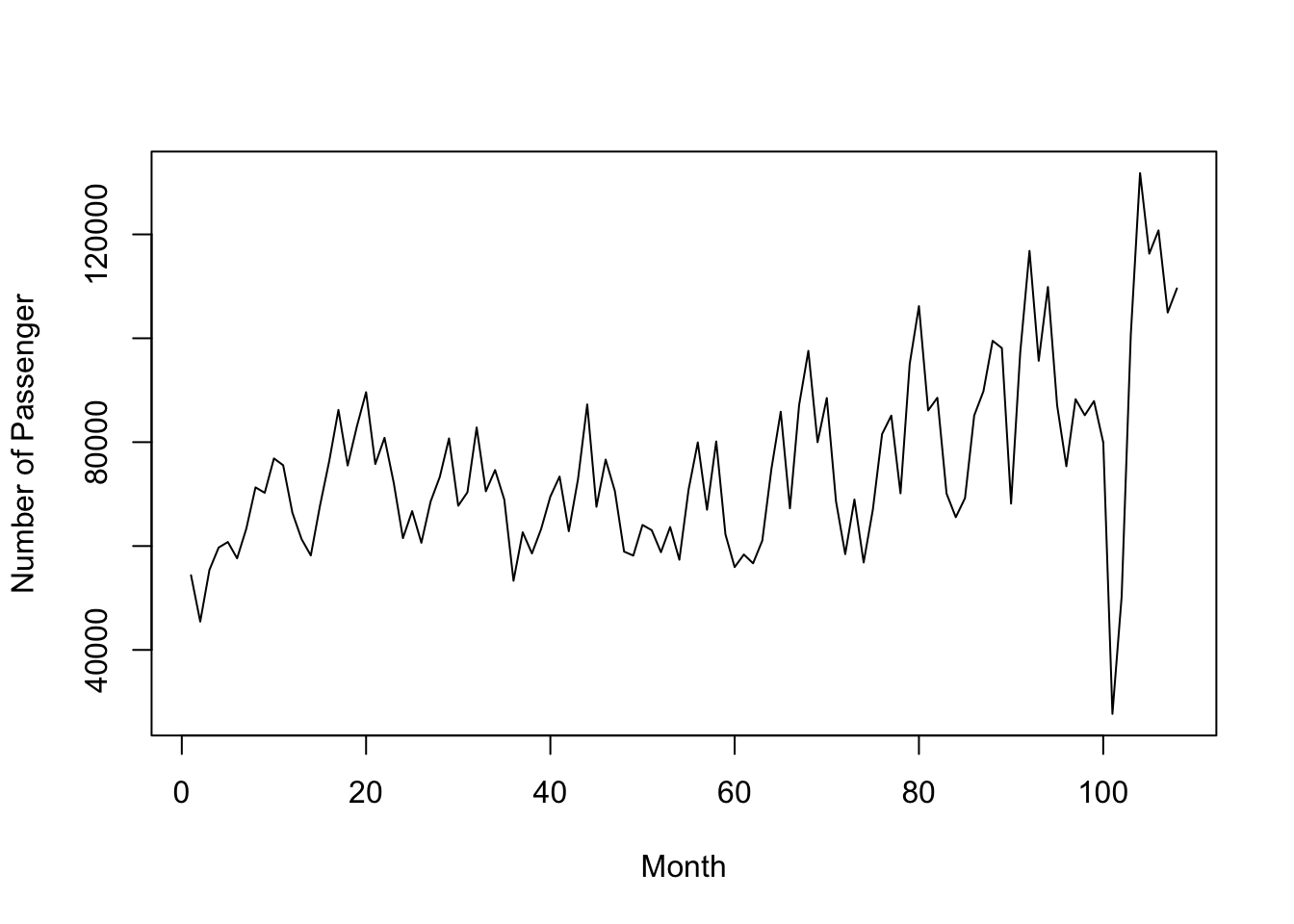

D <- TJair[1:54]-TJair[55:108]
Splus <- sum(sign(D)==1)
Sminus <- sum(sign(D)==1)
K <- min(Splus,Sminus)
pbinom(K,54,.5)

## [1] 0.001919133

2.6 2.5 随机性的游程检验*

判断n重伯努利试验结果是否随机
称连在一起的0或1为游程
游程个数R的条件分布

2.6.0.1 自定义函数

runs.test0=function(y,cut=0){ 
  if(cut!=0)x=(y>cut)*1 else x=y
  N=length(x);k=1;
  for(i in 1:(N-1))if (x[i]!=x[i+1])k=k+1;r=k;
  m=sum(1-x);n=N-m;
  P1=function(m,n,k){
    2*choose(m-1,k-1)/choose(m+n,n)*choose(n-1,k-1)
  }
  P2=function(m,n,k){
    choose(m-1,k-1)*choose(n-1,k)/choose(m+n,n)
               +choose(m-1,k)*choose(n-1,k-1)/choose(m+n,n)
  }
  r2=floor(r/2);
  if(r2==r/2){
    pv=0;for(i in 1:r2) pv=pv+P1(m,n,i);
    for(i in 1:(r2-1)) pv=pv+P2(m,n,i)
  } 
  else{
    pv=0
    for(i in 1:r2) pv=pv+P1(m,n,i)
    for(i in 1:r2) pv=pv+P2(m,n,i)
  };
  if(r2==r/2) pv1=1-pv+P1(m,n,r2) else pv1=1-pv+P2(m,n,r2);
  z=(r-2*m*n/N-1)/sqrt(2*m*n*(2*m*n-m-n)/(m+n)^2/(m+n-1));
  ap1=pnorm(z);ap2=1-ap1;tpv=min(pv,pv1)*2;
  list(m=m,n=n,N=N,R=r,Exact.pvalue1=pv,
  Exact.pvalue2=pv1,Aprox.pvalue1=ap1,Aprox.pvalue2=ap2,
  Exact.2sided.pvalue=tpv,Approx.2sided.pvalue=min(ap1,ap2)*2)
}
run02 <- read.table(file="data/run02.TXT")
(run02 <- run02$V1)

##  [1] 12.27  9.92 10.81 11.79 11.87 10.90 11.22 10.80 10.33  9.30  9.81  8.85
## [13]  9.32  8.67  9.32  9.53  9.58  8.94  7.89 10.77

runs.test0(run02,median(run02))

## $m
## [1] 10
## 
## $n
## [1] 10
## 
## $N
## [1] 20
## 
## $R
## [1] 3
## 
## $Exact.pvalue1
## [1] 5.953799e-05
## 
## $Exact.pvalue2
## [1] 0.9999892
## 
## $Aprox.pvalue1
## [1] 0.0001185775
## 
## $Aprox.pvalue2
## [1] 0.9998814
## 
## $Exact.2sided.pvalue
## [1] 0.000119076
## 
## $Approx.2sided.pvalue
## [1] 0.0002371551

y <- factor(sign(run02-median(run02)),labels=c(0,1))

2.6.0.2 runs.test函数

library(tseries)

## Registered S3 method overwritten by 'quantmod':
##   method            from
##   as.zoo.data.frame zoo

runs.test(y)

## 
##  Runs Test
## 
## data:  y
## Standard Normal = -3.6757, p-value = 0.0002372
## alternative hypothesis: two.sided

第 2 章 单样本位置参数

2.1 引入的例子：楼盘均价

2.2 2.1 符号检验 Sign Test

2.2.1 2.1.1. 广义符号检验

2.2.1.1 SIGN.test只能处理中位数的问题

2.2.1.2 自定义函数：广义符号检验

2.2.2 2.1.2 分位点的置信区间

2.2.2.1 中位数的置信区间

2.2.2.2 自定义函数（一）：中位数的置信区间

2.2.2.3 自定义函数（二）：中位数的置信区间

2.2.2.4 分位数的置信区间

2.3 2.2 Wilcoxon符号秩检验(Wilcoxon Sign Rank)

2.3.1 2.2.1 检验

2.3.2 2.2.2 置信区间

2.3.2.1 Walsh平均

2.3.2.2 利用Walsh平均构造置信区间

2.3.3 simulation study

2.4 2.3 正态记分检验*(normal score)

2.5 2.4 Cox-Stuart趋势检验*

2.6 2.5 随机性的游程检验*

2.6.0.1 自定义函数

2.6.0.2 runs.test函数

第 2 章单样本位置参数